• Motivation
• Computation Technique
• A Better Algorithm
• Results
• Timing

Motivation

Linear regressions have a fairly strict set of assumptions that need to be satisfied to make meaningful conclusions about the p-value or estimation error, such as normality and independence of the residuals. Moreover, many data sets do not satisfy these assumptions, even though many statistics books would have one believe most things are distributed normally. For example, most financial data sets are fat-tailed.

At the expense of producing a predictive model, Spearman Rho is a much more robust test for the existence of a monotonic relationship between the variables. However, the null distribution is more complex, so it's also more difficult to obtain an accurate p-value. (I'd argue an exact p-value is far less important than knowing certainly that the model assumptions hold!) The computation below shows the exact null distribution for small sample sizes.

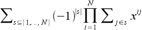
Furthermore, the null distribution is also related to a number theory problem of intrinsic interest: the distribution of , where is a random permutation on the numbers 1 through N, and i ranges from 1 through N. See also A056876.

Unfortunately, until now, there was little data freely available on the internet about this distribution. Several statistics papers have discussed it, but the only free one I can find is here (Fast computation of the exact null distributio of Spearman's rho and Page's L statistic for samples with and without ties, M.A. van de Wiel and A. Di Bucchianico).

Computation technique

Note: I've discovered an algorithm with better complexity but haven't implemented it yet. See the next section for details.

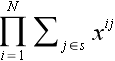
As in the aforementioned paper, a convenient technique for calculating the distribution of , from which one easily obtains the Spearman Rho null distribution, is using the permanent of . One can verify that the coefficient of xⁱ is the frequency for the sum i. So, this computation is equivalent to calculating the permanent of a certain symmetric matrix of monomials.

The paper uses a Laplace-type expansion for the permanent, and then by factoring out powers of x and using symmetry, a great deal of computation can be reused. They do not provide a complexity analysis or timing results, but it appears to be O(2ⁿn⁵) on a cursory look. (We assume arithmetic operations have constant cost. In reality, precision of n log n is required.) It also appears to require a fair amount of memory for the reusable computations, although they do not address this in the paper.

Instead, I opted to use Ryser's formula,

• The product for a subset s+1 is just x^n(n+1)/2 times the product for s. This halves the number of terms needed in Ryser's formula, although its impact is smaller on computation time.
• In the polynomial multiplications, one factor has only coefficients of 0 or 1, allowing a fast and simple implementation with only integer addition.
• Many coefficients do not need to be computed: smaller powers of x are 0 in the final distribution, and the distribution is symmetric so only half needs to be computed. This is a constant factor improvement, about a doubling of speed for symmetry and a 30% boost for skipping smaller powers of x.
  • Symmetry of the products for s and n+1-s could be used, but is incompatible with this optimization.
• Multiplication by a polynomial with only 0-1 coefficients can often be done in fewer operations by reusing intermediate results. For example, multplying by (1 + x + x² + x³) can be done in by multiplying by (1 + x) then (1 + x²), which is faster. There are many possible reductions like this, and a complete factorization isn't necessary for there to be speedups. I have not attempted to implement this sort of optimization, but I thought it was worth mentioning. My intuition is that less than a factor of 2 speedup is possible, but it may be worth further investigation.

My program is a fairly straightforward implementation of the above in C++, no fancy assembly or other low-level coding was used. 96-bit integers were used, which should accommodate N through 30. (Note that intermediate results exceed the 96-bit limit. However, this just means the computation is done modulo 2⁹⁶, and the final result is still valid.) The platform is Win32, compiled with gcc. I may make the source available after cleaning it up, but I would also like to try some other optimizations, such as CPU vector operations.

An algorithm with better complexity

I did also find an algorithm with better complexity. Simply choose O(n³) values for x and compute the permanent. The generating function for the distribution can be recovered using polynomial interpolation techniques. Using an efficient implementation of Ryser's formula, the permanent takes time O(2ⁿn), thus we arrive at complexity O(2ⁿn⁴). Again, this is the number of arithmetic operations; n log n bits of precision are required.

Results

Below are tables of the exact distribution.

• "Sum" is the value of
• "Rho" is the corresponding Spearman Rho value
• "CDF" is the cumulative distribution (useful to convert to p-values)
• "Frequency" is the exact number of occurences of that row's value

Note that the results of a computation are NOT copyrighted. Therefore you may freely use these tables. Of course, a citation would be appreciated.

n = 3
n = 4
n = 5
n = 6
n = 7
n = 8
n = 9
n = 10
n = 11
n = 12
n = 13
n = 14
n = 15
n = 16
n = 17
n = 18
n = 19
n = 20
n = 21
n = 22
n = 23
n = 24
n = 25
n = 26

Timing

The timings are on a 2GHz Core 2 Duo, Win32. All numbers are in seconds. This doesn't particularly follow O(2ⁿn⁵), apparently due to cache and memory effects.